8.2 minutes, and you will understand how most data systems execute joins.

From Spark, Snowflake, to BigQuery, here is how joins are built on

My ultimate goal is to help you break into the data engineering field and become a more impactful data engineer. I'm excited to introduce a paid membership option to take this a step further and dedicate even more time to creating in-depth, practical content.

This will allow me to produce even higher-quality articles, diving deeper into the topics that matter most for your growth and making this whole endeavor more sustainable.

To celebrate this new milestone, I’m offering a limited-time 50% discount on the annual plan.

---

Intro

If you need to write SQL for the paycheck (:D), you might be familiar with the join operations. From the left join to the full outer join, data is normalized into separate tables to streamline the ingest, store, and manage process. When insight needs to be gathered from multiple tables, we join them.

The from clause, the join kind (e.g., LEFT JOIN), the join conditions, and 10 minutes later, the result is returned to us.

The beauty of SQL is that you don’t need to care much about the physical implementation of how SQL is executed. The optimizer will do it.

However, understanding how things work behind the scenes will help us, especially data engineers, to debug and optimize our data workload more efficiently.

And, I think understanding joins is worth our time, given that we encounter them almost daily.

This article will outline the fundamental approach most systems implement for join operations. Then, we will see how these approaches are optimized for OLAP systems, which typically require executing the join on a large amount of data from both tables.

Note: This article focuses on the physical implementation of the join operations, so you won’t find the details of logical join operations like LEFT JOIN or RIGHT JOIN. I believe there are tons of excellent resources on the internet that elaborate on this topic.

---

Before we move on

This article will only cover the equi-join, which combines rows from two tables, using the “=“ operator to compare column values.

I will present the table from the left of the join as the left table and the table from the right as the right table, as I found it intuitive. When reading other resources, you might find that the terms outer table and inner table are widely used.

---

Nested loop join

The basic idea of nested loop join (NLJ) is to have two loops.

The first loop will loop through every record in the left table. For each record, we loop through the right table to compare using the join condition. If the condition is met, the combined row is produced as part of the join result.

The advantage of NLJ is its simplicity and ability to be used without requiring auxiliary data structures like hash tables or data to be sorted.

However, the naive NLJ can be inefficient due to scanning the right table repeatedly.

The Block-Nested Loop (BNL) join is an enhancement that aims to reduce the I/O cost of the naive approach. Instead of processing the left table row by row, BNL reads a block of the left table into a memory buffer.

In the context of databases, a block typically refers to the smallest unit of data that a database management system (DBMS) reads or writes from storage.

Then, the entire right table is scanned once for this left table’s block. All rows within the buffered block are compared against each row of the right table, significantly reducing the I/Os.

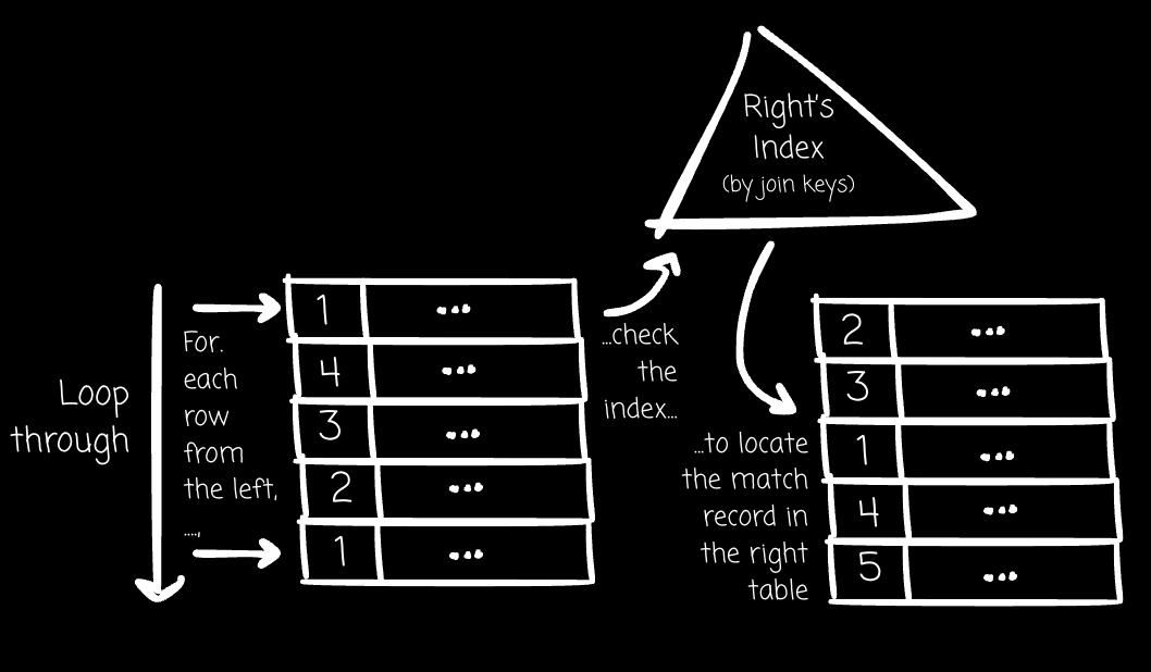
Besides the BNL join, we can use an index to optimize performance. For every record from the left, instead of sequentially scanning the whole right table, the system can check the index to find the location of the matched rows in the right table.

Key takeaways

NLJ can perform reasonably well when the left table is small, which keeps the number of repeat scans of the right table small. In addition, if the right table has an index on the join column(s), the second loop can perform an index lookup instead of a full table scan for each left table row, drastically improving performance.

---

Sort-merge join

The next approach we will explore is the sort-merge join (SMJ)

With SMJ, the system must carry out two phases.

• In the first phase, the system sorts the two tables based on the join columns.

• In the second phase, the system walks through the tables with associated pointers:

  • If the join conditions match, the rows are combined. If duplicates exist in one or both tables for the current join key value, all combinations of matching rows must be generated. This might involve moving the pointer from one table backward while moving the pointer from another forward.

  • If the join values from the left are less than those of the right, the left’s pointer is moved forward.

  • If the join values from the right are less than those of the left, the right’s pointer is moved forward.

  • This process continues until one or both tables are exhausted.

Compared to the NLJ, the system must perform extra sort operations on the two tables. SMJ is particularly efficient when one or both input tables are already sorted on the join columns, or if they have clustered indexes on these attributes, as this can eliminate or reduce the cost of the sort phase.

With a clustered index, the database sorts and stores the rows physically using the values from the index columns.

It is also convenient if the query output must be sorted by the join key ( ORDER BY clause on the join key), as the merge phase naturally produces sorted output.

---

Hash join